AutoSum in the Formulas in Excel 2010
As an alternative, nothing prevents you from typing the correct expression in the Formula Bar; but dragging the desired cells may be visually easier to track. Then press Enter, and all the desired cells are added. (Don’t, by the way, accidentally over-drag into cell C25—because that cell contains the formula itself, and you can’t incorporate it into its own result. That kind of miscue is called a circular reference (and Excel will deliver an onscreen error message to you to that effect), whereby the cell adds itself, as it were—and that causes way too many problems).
Thus we see that the initial range drawn up by AutoSum is merely a friendly suggestion, yours to accept or reject, and one you can replace with a different range if events warrant.
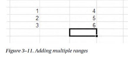
And along these lines, suppose you wanted to add the numbers in Figure 3–11, deposited in cells C14:C16 and E14:E16 respectively:
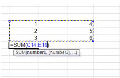
 First, we need to decide the cell in which we want our answer to appear. In the interests of simplicity, let’s choose cell C17. We click AutoSum, and are presented with the range selection seen in Figure 3–12, of course:

Now we have a decision to make. Because we want to add both ranges, we could next drag across all the cells in question, as in Figure 3–13:

Figure 3–13. Kind of a drag: spanning two ranges to be added in one SUM. Note, however, that the function treats these values as one range for formula purposes: C14:E16 And that’s what you probably would do, after which you’d press Enter and return your answer. But suppose there were an additional set of numbers in those in-between cells D14:D16—and you don’t want these incorporated in your answer. If we proceed with the range selection we’ve just named— C14:E16—the numbers in D14:D16 will be brought along, because they too inhabit the selected range.
So how do we exclude these unwanted cells? We can do the following:
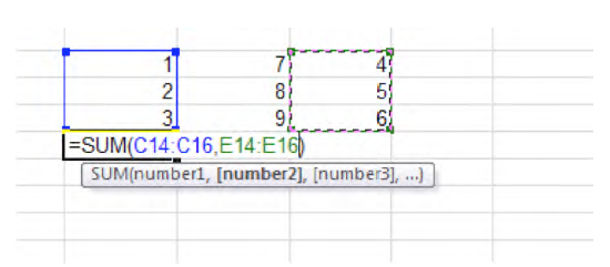
Click AutoSum, yielding the initial C14:C16 range selection. Then type a comma (don’t add a space) and drag range E14:E16 (you can also hold down the Ctrl key after selecting the first range, and then select E14:E16 (Figure 3–14):

Figure 3–14. Adding two ranges-here the two sets of values are treated as two distinct ranges. Then press Enter.
You get the picture. The comma splices our cell selections into two distinct ranges, thus leapfrogging the D14:D16 cells. We’ve now learned a deeper truth about SUM, one that can be projected to all functions: you can identify any cell or range(s) you want in any formula, and place your formulas in any cell in the worksheet (so long as the formula isn’t dropped into the very range you’re referencing in the formula).
Remember that AutoSum was devised in order to execute a simplest-case scenario, the spreadsheet equivalent of a hanging curveball—that classic, add-one-row-or-one-column chore, where the row or column to be added consists of a range, all of whose cells are filled with numbers. But your formula requirements may be more nuanced, and the reality is that you can recruit cells and ranges from all across the worksheet—and even beyond it, as remains to be seen.
Note as well that nothing whatever stops you from typing SUM if you’re so moved, or any other function in Excel, for that matter. As long as you know the syntax, you’re free to tickle the keys as wish; and as we’ll see, Excel offers you a number of ways to see to it that whatever you’re writing turns out correct.
And here are some AutoSum shortcuts: The keyboard equivalent for calling up the command is Alt+=. And if you’re working conventionally, and you know you want to add a standard range of consecutive numbers in a column: just click in an empty cell at the foot of the column and double-click the AutoSum button (as it appears in either the Home or Formulas groups).
Double-clicking cuts immediately to the answer, without requiring you to make any additional range decisions.
And one more observation about AutoSum: if you rest your mouse over either of its buttons, the resulting caption tells you that AutoSum helps you “Display the sum of the selected cells directly after the selected cells”. But we know that isn’t quite true; as we saw earlier you can leave some space between the numbers (as long as these are consecutive) and the formula itself in that column or row and still get AutoSum to work for you, though those empty cells will also be referenced in the formula.
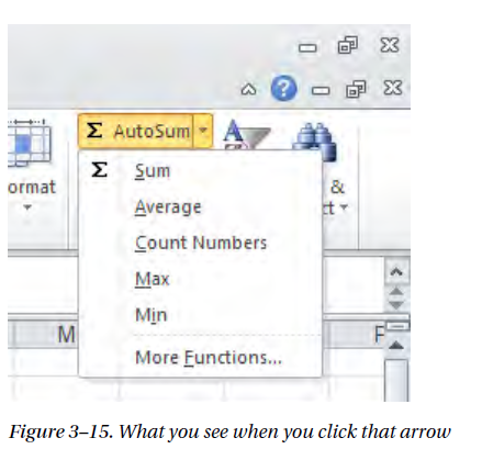
Now, you’ll note that both AutoSum buttons on either tab are accompanied by one of those dropdown arrows we alerted you to a good many pages ago (Figure 3–15):
