Entering Text: Trespassing Allowed in Excel 2010
There is, as is usual with the Office programs, more than one way to do this. The two easiest and fastest are carried out as follows: With your mouse, move up to the right boundary of the column you wish to widen (and not row 1). What started out as Excel’s familiar thick white cross—the one you see when you move about the worksheet proper—should now appear as the slender, black, double-arrowed object seen in Figure 2– 20:
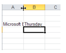
Figure 2–20. The A column, selected for widening You must bring about that double-arrowed pointer in order to widen the column; but it should appear automatically as soon as your mouse arrives atop the right boundary. Then click the boundary, and drag to the right (don’t release the left mouse button). As you do so, the column should expand, revealing ever more of the text. And as you drag, a caption accompanies the action, tallying the current column width both in units of text characters and pixels (this bit of information is usually of little more than academic importance most of the time; just bear in mind that the default width of an Excel column is set at 8.43 characters, for historical reasons). When you’ve achieved the desired width—presumably after all the hidden text has been brought to light—you can release the mouse. Nothing stops you from widening—or narrowing—the column again, by dragging it again to the right or even to the left. If you’ve accidentally clicked on the left boundary of the column you want—which is, after all, the right boundary of the column to its left—then that column will be widened instead.Bring your mouse to that same right column boundary, make sure the double-arrowed cross is in view, and this time double-click. The column will automatically resize itself to reveal all the data in the column. Known as Autofit, this rather efficient device is a time-honored means for solving the hiddentext problem. Note that Autofit modulates the column to make sure to reveal what is currently its widest entry, fitting itself snuggly to that entry’s width; and so if you delete that item from the column and perform another Autofit, the column may narrow, as it hugs what is now the widest entry.
Now for an important variation on the Autofit theme, here’s a scenario you might very well have to confront. Suppose you’ve entered the months of the year, and your data look like Figure 2–21:

Figure 2–21. Columns in need of widening—or narrowing The problem is clear: some of the longer month names have barged into the cells to their right, and these happen to be occupied by months of their own. Thus the same column-width issue emerges; but what’s new here is that we can conduct an Autofit on several columns at the same time.
To make this happen, click the first of the column headings—A—hold the mouse button down, and drag across the remaining headings (again, don’t drag across row 1 on the worksheet; you need to select the headings). Your worksheet would look something like this, as shown in Figure 2–22:
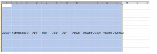
Figure 2–22. Columns selected and prepared for autofitting That blanket of blue cells teaches us incidentally that when you click a column heading, all the cells in that column are selected; but what interests us here is the column width question; so now doubleclick any one of the boundaries separating any of the selected columns, e.g., the one separating B and C, or J and K (again, you’ll need to see that double-arrow cross). All the columns should now be resized, with each new width reflecting the respective widths of the months. See Figure 2–23:

Figure 2–23. Autofit: one size doesn’t fit all It’s a nifty way of Autofitting lots of columns in one go; but now you may have to contend with another possible problem. Thanks to Autofit we can now see all the text, but since each of the months exhibits a different width, so then do the columns housing them—and presentationally speaking, that may not look very nice. You may want uniformly widened columns instead, but you can’t get there from here using Autofit. What to do? The answer is to select all the column headings as described above, but this time, instead of doubleclicking any boundary, we click the right column boundary of the longest month—in this case “September,” given the font being used—and drag a bit to the right. Then release the mouse.
This technique—really a variation on the first column-widening approach we cited earlier—equalizes the width of all the selected columns; and because we dragged on the widest month’s column, naturally all the other months should be visible as well.
And if you drag and release the mouse too soon and fail to reveal the word “September” in its entirety, note that all the columns remain selected, so you can resume dragging until the word is completely exposed.
You’ll also want to know about another data entry option, one you’ll have difficulty ignoring in any case. If you enter text down consecutive cells in a column and have occasion to enter the same datum (that’s the singular, believe it or not) twice in different cells, Excel will automatically enter it for you the second (and every subsequent) time in the cell in which you’re typing, as soon as it recognizes it. That is, if you enter “John” in cell D2 and “Bill” in D3, and then begin to enter “John” in D4, Excel will complete the name “John” as soon as you type the letter J (this will happen even if you type a lower-case j. See Figure 2–24:
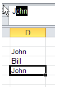
Figure 2–24. AutoComplete in action; note the formula bar That is, Excel will try to AutoComplete the name. If you approve f the suggestion, simply press Enter. But if you really want to type “Jerry” in D4, just keep on typing. Note that if you’ve already entered “Mary” and “May” in different cells, you’ll need to type the third letter in either of these names, as Excel won’t otherwise know which name you wanted to AutoComplete. But again, if you want “Martin” instead, keep on typing.
But what is entirely possible to ignore is another, related feature. Once you’ve typed even one name with the intention of continuing to type down a column, you can right-click the next cell, and take note of this option in Figure 2–25:
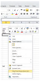
Figure 2–25. Your on-the-fly drop-down list in the making…If I click here, the menu shown in Figure 2–26 appears:
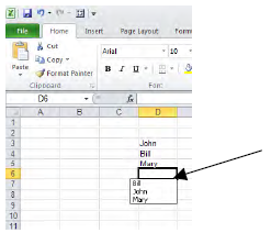
Figure 2–26. …and here it is It’s a mini-drop-down, grabbing its data from the current list of names you’ve typed in the list to date—and the list incorporates any new names as you type them. Just click one. Cool, and little known.