More of the Same in Excel 2010 Part 2
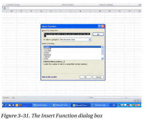
While the buttons in the Function Library afford the most up-front way in which to access functions, Excel makes other ways available, too. You can also click the fx button flanking the Formula Bar to its left and call up this dialog box (Figure 3–31):

In fact, this Insert Function box does nothing more than enumerate the same contents of the respective Library buttons. Click the Or select a category drop-down arrow and you’ll see the identical categories by which the Library buttons are classified.
Then click a category and any of the function names that appear next, and you’ll be returned to exactly the same function Arguments dialog box we witnessed a few screen shots back..
And take note of the Formulas tab’s Insert Function button. Click it and, well, you’ve done nothing more than tap a giant-sized twin of the fx button. Is this button redundant? Probably.
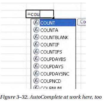
But there is another, decidedly different way to requisition the function you want. Click the cell in which you’re working, type =, and begin to enter the function name. As you type, an AutoComplete mechanism activates, presenting and narrowing a list of functions beginning with the letters you’ve typed. Type more letters and the list shrinks, as shown in Figure 3–32:

When you see the one you want, you can either double-click its name, or scroll down to the function in question with the Down arrow key and press Tab (but not Enter). You’ll see, for example (Figure 3 – 33):

Then start to type the remainder of the functions. True, you’ll have to know what to type next, but that’s going to come with repetition. (Note the small caption that offers a kind of running commentary about which argument you’re currently entering between the parentheses, e.g., which number range you’re now identifying in COUNT. But don’t worry—more on arguments soon).
The first thing you want to know about functions and formulas (remember that functions are builtin Excel formulas) is that they can be mixed and matched in innumerable ways. They needn’t be composed and applied in isolation, and can be related to each other in the same formula, and for a myriad of purposes. So start priming that spreadsheet imagination.
For example, consider this formula: =AVERAGE(B3:E3)+5 This could, for example, be used to calculate a student’s average for four exams (spanning columns B through E), to which 5 points are added—as a kind of bonus.
Now how about this? =MIN(B3:E3)*1.05 We’re working with same four tests. Here our beneficent instructor is adding 5 percent to a student’s lowest—that is, minimum—score. Not five points, mind you, but 5 percent. Thus if our student bombed test number 3 with a 58, the above formula will take that score and multiply it by 1.05, coming up with 60.9. Of course, if our teacher is as beneficent as we say, she’ll round it up to 61. Note, by the way, that both of these formulas factor in both a function and an actual, garden-variety number. That’s part of Excel’s mix-and-match capability.
Now think about this one: =(SUM(B3:E3)-MIN(B3:E3))/(COUNT(B3:E3)-1) True, this one looks scary—at least at first, and perhaps even second perusal. But in reality, it doesn’t introduce any feature that we haven’t already learned. What this formula does is add the scores of all four exams, and subtracts from that total the lowest score. It then divides this new result by the number of remaining exams, that is, 3. In effect the formula calculates the average of the three highest exam scores, having dropped the lowest score.
Let’s look at this one more closely—and I’ll submit the hope that, upon reflection, you’ll agree the formula isn’t quite as daunting as you may suppose.
Let’s assume our student has scored 76, 82, 58, and 91 on the quartet of exams. Note the entire formula as usual begins with an = sign. But then note that a pair of parentheses surrounds both the SUM and MIN parts of the formula together, this in addition to the parentheses surrounding the individual ranges identified in SUM and MIN. Thus observe the two consecutive parentheses following the B3:E3 range reference in MIN. One simply serves as the closing parenthesis in MIN’s own range; the other bounds off the combined SUM-MIN expression, thus letting us compute this total: 76+82+58+91-58 Or 307-58, which equals 249. And why then do we need this pair of global parentheses around SUM and MIN? Because of the order of operations, which assigns priority to expressions surrounded by those parentheses, allowing us to treat the activity going in between them as one unit.
And once we derive it, that 249 is ultimately to be divided by 3—that is, the number of exams minus 1. Now take a look at our divisor:
(COUNT(B3:E3)-1) And guess what—this expression is also surrounded by parentheses, and for exactly the same reason—the order of operations. Remove those outside parentheses and our divisior would read, formulaically:
COUNT(B3:E3)-1 and numerically: 249/4, then minus 1. The result: 61.25. But bring back those outer parentheses and you get: 249/(4-1) or 83, the number we want.
As a matter of fact , if we peeled off the global parentheses on both sides of the divisor, our formula would stand as:
=SUM(B3:D3)-MIN(B3:D3)/COUNT(B3:D3)-1
And that would yield us 291.5, not even close to the number we want. Try it and you’ll see.
Thus writing formulas involves thinking your objectives through, fooling around with practice formulas, making mistakes, and learning from them—and lining up those parentheses when you need them (and Excel will be sure to notify you with an error message when the count of your open parentheses doesn’t equal that of your closed ones, something like “Microsoft Excel found an error in the formula you entered,” and will offer you a corrected suggestion. Click No to the suggestion and you’ll be sent another message, observing that your expression as it stands is missing a parenthesis).
A final note on the above exercise. Even though our formula made important use of the SUM function, we’d probably be advised not to write it and not to click the AutoSum button in order to post it to its cell. And that’s because SUM deoesn’t stand alone in its cell this time; we needed to continue to type additional characters (incuding that first global parenthesis before the word SUM, which you won’t get by clicking AutoSum) in order to combine SUM with the additional formula elements. Just remember, though, that you can always type any function if you need or want to; and in this case, you could type: =(SUM( and at that point drag the range B3:E3, continue to type: )-MIN( and then drag B3:E3 in order to identify that range for MIN, and continue to type. (And remember that when you begin to type a function name, the Auto Complete menu will appear.) Now thus far we’ve confined our discussion of functions to the ones that are presented to us on the AutoSum drop-down menu. But as we stated earlier, there are hundreds more. Time and space will restrict our treatment here to just a few of them, but once you get the general hang of these things.