Not Just Your Average Function in Excel 2010 Part 4
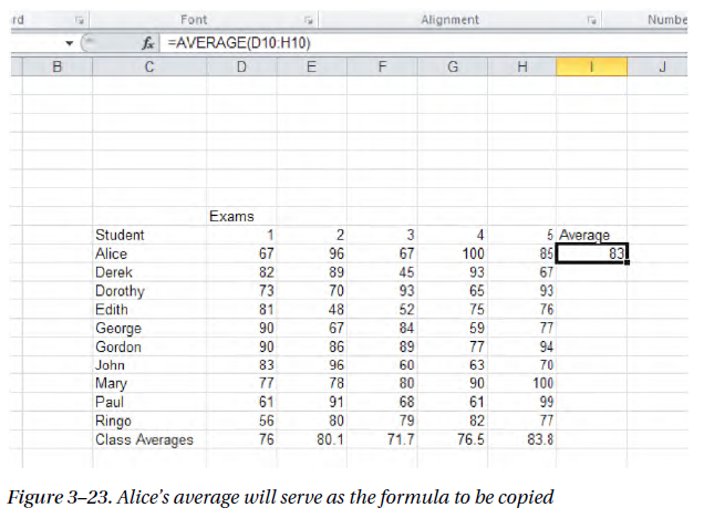
We see, then, that the 7 won’t change—only the original D5 will. And when you need to copy a formula containing cell references down a column or across a row, there’s a most expeditious way to do so, by finding a novel use for a tool we already know —the fill handle. To illustrate: Let’s take a few steps back in the design of our grading sheet, and for the sake of clarity, we’ll scrub away all the fancy formatting, too. We’ve written Alice’s AVERAGE formula, and now want to copy it down the column, as in Figure 3–23:

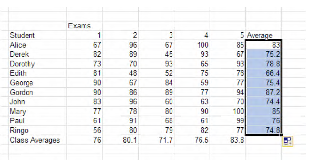
If I station my mouse over the fill handle in cell I10—Alice’s test average—and then click the handle, don’t release the mouse, and drag down the column through Ringo’s cell in cell I19 and then release the mouse, I will have copied all the student AVERAGE formulas, as in Figure 3–24:

Figure 3–24. Copying allowed, here: Dragging to copy Alice’s formula gives me the averages for all the students Then click anywhere to turn off the blue selection color. Here, the fill handle—that same device we earlier put to the task of producing series of data—e.g., 1,3,5,7, days of the week, etc.—is used to copy formulas. Just click on the first (which at the moment is the only) formula, and drag the fill handle as far as you need to go—either down a column or across a row. The copy procedure collaborates with relative referencing to install the proper cell references in each cell, and what this means is that if you need to copy a formula to many cells, you only need to actually write the formula once—the formula that will serve as the model to be copied to all other cells.
And once you learn how that capability works, there’s an even easier and cooler means to carry out this kind of copying task.
nce you write that first, model formula, click back on that cell (in this case Alice’s average in I10), and double-click the fill handle. All the other student cells running down the I column receive the formula, without you needing to drag the fill handle.
he double-click automatically copies the original formula down all the cells that also have data in the immediately adjoining column to its left or right.
To summarize this tip—if you need to copy a formula down a column—and this only works when you copy down a column, not across a row—click on the cell storing the original formula and then double-click its fill handle. As long as there are data in the adjoining column (either to the left or right; and that means in our example if the H column were empty this wouldn’t work), the formula copies down for as many rows as there are data. And this will work as surely for 20,000 rows as it will for 20. I use this shortcut all time; I told you I was lazy.
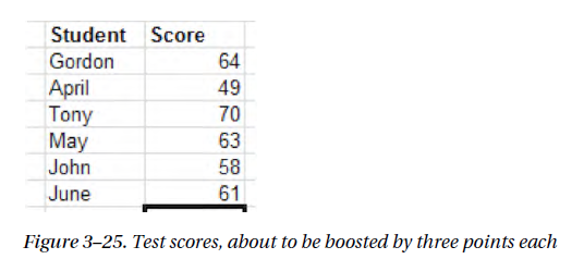
Now there is one more permutation of this cell-reference copying business that you need to know. Consider this case: Suppose I’ve given my students a rather challenging exam, and, after having canvassed the sobering results, decide to grant them an extra three points in order to curve the scores upward. My simple grade book looks like Figure 3–25, at the outset:

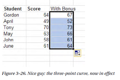
So how do I go about padding these pause-giving scores by those three points? Gordon’s score is in cell D11, and so I could write the following in E11, couldn’t I: =D11+3 Sure I could. Then I’d return to cell E11, and utilize my newfound double- click-on the fill-handle trick.
I’ll bring about this revised grade distribution (Figure 3 – 26):

Are my calculations correct? Absolutely; but still I wouldn’t recommend this approach. That’s because if I conclude that I need to award my charges say, 5 points instead, I’d need to edit the formula in E11 to read: =D11+5 and then copy that rewritten expression down the column again, so that all the students will enjoy my 5- point largesse. Not an enormously big deal, but not an elegant way in which to proceed. As a rule, one wants to avoid editing cells if one can; it can get messy, and a preferable alternative would be to enter the 5-point bonus figure in a cell—say in this case, A11, and rewrite Gordon’s formula thusly: =D11+A11 and copy it down the column. And exactly why is this approach recommended? Because if I change my mind again and issue a 7-point curve, all I need do is type 7 in cell A11, and all the scores should change automatically—with no additional cell editing required.