More of the Same in Excel 2010 Part 3
Let’s start with VLOOKUP, a function I’ve used countless times to do countless things. The V in VLOOKUP stands for vertical and points to what’s called a lookup table, a collection of data in which a value is….looked up.
But that’s terribly abstract. Let’s look at a VLOOKUP example, turning once again to the real-world domain of exam grading.
Suppose I’ve been entrusted with one more batch of grades, to which I assign numerical scores which must be converted into letter grades. In cells K10 through L14, establish the scale shown in Figure 3–34:
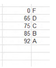
Figure 3–34. Another lookup table, featuring a grading scale It’s a rather simple affair, but notice what the table seems to require, and not to require. The table reads vertically, naturally, and in our case consists of two columns, the first of which records a series of grade intervals which are arrayed in ascending order and aren’t evenly spaced in equal numeric intervals—that isn’t required.
The second column enumerates the alphabetic grade equivalents, each one of which represents a grade threshold. For example, in order to earn a B you need to achieve a minimum score of 85. Score an 84, and you get a C. Score an 84.9, and you get a C. Tough teacher.
Now we’ll enter the scores to be looked up and assigned those alphabet grades. We’ll just work with five students, so in cells A10:B14 enter (Figure 3–35):
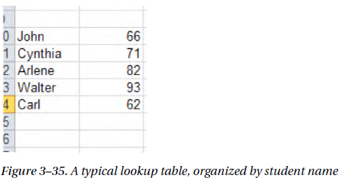
And it’s in the C column, alongside each student grade, in which we’ll compose our VLOOKUPs. Click in cell C10 and type:
=VLOOKUP(B10,K$10:L$14,2,TRUE) .
Don’t worry—we’re going to explain all this. First note the constant elements we’ve spoken about earlier: the equal sign, followed by the function name and an open parenthesis. Second, we see that, unlike say, COUNT or AVERAGE, something more than just a range is fitted in between the parentheses.
Here four different elements—or arguments, and we’ve spoken about them, too—have creeped in there.
The first—in this case B10—names the cell whose grade is going to be looked up and assessed. That’s John’s 66. The second argument—K$10:L$14—pinpoints our lookup range itself, and yes, it’s accompanied by those dollar signs, slipped in before the 10 and the 14—the row segments of two cell addresses. And why? Because we want to look up all our students’ grades in the same lookup table again and again, and we intend to copy K$10:L$14 down the column of students without its cell references changing.
The third argument—2—refers to the column in the lookup table containing the “answer”—that is, John’s alphabetic grade; and so what VLOOKUP does next is this: it takes John’s 66 (in B10) and compares it to the numeric grades in the first column of the lookup table—that is, the K column. John’s 66 falls between the 65 and the 75 in that column, whereupon VLOOKUP treats it as the lower of these two values (remember—these are grade thresholds, and John hasn’t reached 75), and it then looks to see which grade has lined up with 65 in the lookup table’s second column—in this case, D. That’s the 2 in the third argument. John gets a D, and we can now copy this formula down the C column (using that nifty fill-handle double-click if we wish, because all the cells in the adjoining B column have data in them).
he fourth argument—TRUE, which would have been assumed by default anyway even if you hadn’t written it—provides for what’s called an approximate match. It’s this argument which allows VLOOKUP to assess each numeric grade and find its grade niche, e.g., a 78 falls between the lookup table’s 75 and 85.
Once done, the student grades should read (Figure 3–36):
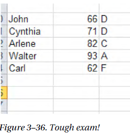
and of course this process would enable us to assign the grades of 5000 students, too, not just 5. And note importantly that the lowest grade we’re able to look up in this table is 0 (the entry in K10). Even if it’s unlikely that any student will score that poorly, you want your table to be able to handle all contingencies—because had I entered a lowest-possible test score of say, 30, in K10 instead and the hard-partying John crashes and burns with a 25, that score would yield an error message in his VLOOKUP. You can’t look up a score below the lowest value in the lookup table.
Let’s demonstrate another instance of VLOOKUP, and then review. Suppose we want to calculate some income tax obligations (purely hypothetical, you understand). We can draw up this tax lookup table in cells B8:C18 (Figure 3–37):
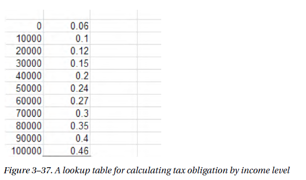
The table presents a tax schedule, which assesses income in dollars, and the values in the second column are really percentages. I haven’t formatted either column as currency and percent, respectively, simply because we haven’t gotten to formatting yet. Thus an income of $32,567 would be assessed at a rate of .15, or 15%, because that income falls between 30000 and 40000, and again VLOOKUP falls back to the lower of the two and “looks up” the matching figure for 30000 in the second column : .15. In H8 we can enter any income total, say 62789, and in I8 we can write:
=VLOOKUP(A8,B8:C18,2,TRUE) .
Our answer: .27, or 27%.
There’s nothing conceptually new in this second case—it’s pure review. VLOOKUP takes the number in cell H8-62789—and compares it to the values in the first column of the lookup table in B8:C18. Because the income falls between 60000 and 70000, it’s treated as the former, whereupon 60000 is measured against the same row in the second column—namely, .27.
And where are the dollar signs, you ask? You could enter them, and you would, if you had a string of incomes to assess down the H column starting with H8. You’d then copy the original VLOOKUP in I8 down the I column, and yes—here the dollar signs would be most handy indeed, because we’d want all the incomes to be looked up on the same table.
As usual, there’s more to say about VLOOKUP. For one thing, if you wanted to learn exactly how much tax a taxpayer actually owes, we could write in cell I8: =VLOOKUP(A8,B8:C18,2,TRUE)*A8 See how that works? It looks up 62789, yields .27, and goes on to multiply 62789 by .27, returning: $16,953.03 Once the formatting is applied.
Some other VLOOKUP thoughts: note that our lookup tables to date have comprised two columns.
But nothing prevents us from adding a third and even more columns, which would enable us to achieve different sets of lookup outcomes.
For example, I could devise this lookup table, if we return to our grading chores (Figure 3 -38):
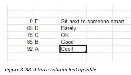
And we could rewrite John’s VLOOKUP in C10 to read: =VLOOKUP(B10,K$10:M$14,3,TRUE) In which case we’d see Barely in that cell.
And what’s different about this rewrite? Two things: the lookup table now spans three columns, and we’re we’re looking up our “answer”—the item which will appear in C10—in that third column.
One more VLOOKUP permutation: Suppose we wanted to be able to type a student’s name in a selected cell and be able to immediately determine the numeric grade she earned. That is, if I type Cynthia I want to see 71 in the next cell, and so on. If so, we could treat our student name/grade list— A10:B14—as a lookup table. Why not?
And in D10 we could enter any student’s name, and in E10 write:
=VLOOKUP(D10,A10:B14,2,FALSE)
I see I can’t put anything by you. You’ve noticed a new, fourth argument in that formula, and here’s why.
By default, VLOOKUP requires that the first lookup table coluum—the one containing the values to be looked up and assessed—be arrayed either in ascending numerical or alphabetical order (yes; that first column can display text). But we see that the first column in our current lookup table—the names of students—are assuredly not in such order. If we don’t want to sort the list—and here we don’t—we can enter FALSE in the VLOOKUP syntax, which instructs Excel to look for exact matches in the first column, irrespective their order—no more approximate matches. So if I type Cynthia in D10, I should see 71 in E10. If I omit the FALSE, I won’t see 71 there. And if I type Barack in D10—a name which doesn’t appear at all in the lookup table—I’ll get an error message.